February 23, 2017 / by / In deeplearning

Deep Learning 101 - Part 2: Multilayer Perceptrons

tl;dr: What to do when you have standard tabular data. This post covers the basics of standard feed-forward neural nets, aka multilayer perceptrons (MLPs)

The Deep Learning 101 series is a companion piece to a talk given as part of the Department of Biomedical Informatics @ Harvard Medical School ‘Open Insights’ series. Slides for the talk are available here and a recording is also available on youtube

Other Posts in this Series

• Part 1: History and Background

Introduction

In this post we’ll cover the fundamentals of neural nets using a specific type of network called a “multilayer perceptron”, or MLP for short. The post will be mostly conceptual, but if you’d rather jump right into some code click over to this jupyter notebook. This post assumes you have some familiarity with basic statistics, linear algebra, calculus and python programming.

MLPs are usually employed when you have what most people would consider “standard data”, e.g. data in a tabular format where rows are samples and columns are variables. Another import feature here is that the rows and columns are both exchangeable, meaning we can swap both the order of the rows or the order of the columns and not change the ‘meaning’ on the input data.

MLPs are actually not responsible of most recent progress in deep learning, so why start with them instead of more advanced, state of the art models? The answer is mostly pedagogical, but also practical. Deep learning has developed a lot of useful abstractions to make life easier, but like all abstractions, they are leaky. In accordance with the Law of Leaky Abstractions:

All non-trivial abstractions, to some degree, are leaky.

At some point the deep learning abstraction you’re using is going to leak, and you’re going to need to know what’s going on underneath the hood to fix it. MLPs are the easiest entry point and contain most (if not all) of the conceptual machinery needed to fix more advanced models, should you ever find yours taking on water.

Logistic Regression as a Simple Neural Network

Note: Hop over to the corresponding jupyter notebook for more details on how to implement this model

Hey! I thought this was about deep learning? Why are we talking about logistic regression? Everyone already knows about that.

Great question! Here is a cookie for you! Most people are familiar with logistic regression so it makes a sensible starting point. As we will see, logistic regression can be viewed as a simple kind of neural network, so we’ll use it to build up some intuitions before moving to the more advanced stuff.

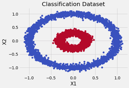
Assume that we’ve collected data and would like to build a new classifier. To be concrete, pretend that we’ve gathered up data where each sample has two variables, $\{x_1,x_2\}$ and an associated class label that tells us if it is a “blue dot” or a “red dot”. When we plot our data, we see a picture like this one:

Let’s formalize our notation a bit and represent each observation as a vector of 2 variables $x_i = <x_{i1},x_{i2}>$ and convert our class labels of “blue” and “red” to a binary variable called $y_i \in \{0,1\}$, where $blue = 0$ and $red = 1$. Now we want to construct some function, let’s call it $f(x_i)$, to model the relationship between $x_i$ and $y_i$ so that when we get new data, we can correctly predict if it’s a blue dot or a red dot. The most straight-forward way to construct $f(x_i)$ is weight each variable and add them up in a linear model:

$$f(x_i) := w_0 + x_{i1} * w_1 + x_{i2} * w_2$$

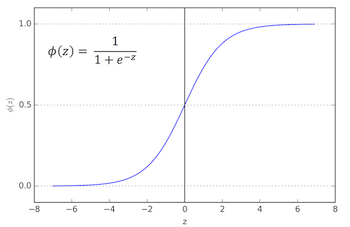
where each $\{w_1,w_2\} \in \mathbb{R}$ is a scalar that weights the contribution of each variable, and $w_0$ is the intercept term. So $f(x_i)$ takes each variable, performs a weighted-sum to create a single real-valued number that we’d like to compare to our outcome variable, $y_i$. Since our outcome is binary, we can’t directly compare it to $f(x_i)$, since our function can take on any number on the real line. Instead, we’ll transform $f(x_i)$ so that it represents the probability $y_i = 1$. To do this we will need to introduce a function known as a logistic function, called $p(x_i)$:

$$p(x_i) := \frac{1}{1 + \exp(-f(x_i))}$$

$p(x_i)$ represents the conditional probability that $y_i$ is a 1, given the observed values in $x_i$, i.e. $Pr(y_i = 1 \mid x_i)$. This perhaps strange looking function takes the number created by $f(x_i)$ and ‘squashes’ it be between 0 and 1, and gives us the conditional probability that we’re interested in. The graph of the sigmoid is shown below, with $f(x_i)$ on the x-axis and $p(x_i)$ on the y-axis:

Why should we prefer this specific function over potential alternatives? After all, there are many ways to squash a number to fall between 0 and 1. For one, it has a very nice and easy to compute derivate and it has a variety of nice statistical interpretations, yields interpretable quantities known as odds-ratios, but for now let’s just roll with it.

So we’ve defined a model $f(x_i)$, linked it to our target variable using the logistic function, and now we just have one more piece we need to define. We need a way to “measure” how close our predicted value, $p(x_i)$, is to the true value $y_i$. This is known as a loss function, represented as $\mathcal{L(.)}$. The most common choice for a loss function in a classification task like this is binary crossentropy (BCE), shown below:

$$\mathcal{L}(y;w) := -y_i * \log(p(x_i)) - (1-y_i) * \log(1-p(x_i))$$

This function is low when $p(x_i)$ and $y_i$ are similar and is high when they are dissimilar. For example, if $y_i = 1$ and our predicted probability is $p(x_i)=0.9$ then the loss function takes a value of $0.105$. However, if we instead had a predicted probability of $0.1$ the loss function would have a value of $2.3$. Again, why is this a sensible choice for a loss function? Well, there are a few reasons including again a nice derivative, but BCE also happens to be the negative log-likelihood (NLL) of a Bernoulli random variable. Since our task is predicting a binary outcome, using the NLL of a Bernoulli random variable seems like a sensible thing to do.

To recap: We’ve defined our model, $f(x_i)$, converted it to be on the same scale as our response using the logistic transformation, $p(x_i)$, and decided on a way to measure how good our predictions are using the binary crossentropy loss function, $\mathcal{L}(y,p(x_i))$.

So, how do we actually learn values for $\{w_0, w_1, w_2\}$ that minimize $\mathcal{L}(y,p(x_i))$? Enter Stochastic Gradient Descent (SGD).

Stochastic Gradient Descent (SGD)

Imagine for a moment that you have been left blind and stranded on the side of a mountain. How would you get down? Underfoot you can feel that the direction of steepest descent is approximately $35^\circ$ to your left, so you pivot and take a step in this direction. You gather yourself, feel again and take another step according to the local slop of the mountain. Once the ground feels level, you conclude that you’ve probably reached the bottom, or at least a plateau.

This procedure is exactly how SGD finds parameter values to minimize a loss function. Instead of tactile input, SGD computes the derivative of each parameter with respect the loss function and takes a small step in the opposite direction (e.g. negative gradient). So we need to analytically compute the derivative for each weight in our model, so that we know how to iteratively update it to improve our predictions. To keep things simple, we’re just going to derive the update for $w_1$, but it’s almost exactly the same for the other parameters. Recall, the chain rule tells us how to compute derivatives for a composed set of functions, which is exactly what we have here. What we really want is the partial derivative $\frac{\partial \mathcal{L}}{\partial w_1}$, but we have to use the chain rule to peel off some of the layers of this functional onion first. The roadmap looks like this:

$$\frac{\partial \mathcal{L}}{\partial w_1} = \frac{\partial \mathcal{L}}{\partial p_i} \frac{\partial p_i}{\partial w_1}$$

So we start simply, by computing the first term:

$$\begin{aligned} \frac{\partial \mathcal{L}}{\partial p_i} = -\frac{y_i}{p_i} + \frac{1-y_i}{1-p_i} = \frac{p_i-y_i}{p_i(1-p_i)} \end{aligned}$$

Next, we compute the second term:

$$\begin{aligned} \frac{\partial p_i}{\partial w_1} = p_i*(1-p_i) * x_1 \end{aligned}$$

which was made simple by the nice derivative property of the logistic function. Now, we combine the two to get the full derivative:

$$\begin{aligned} \frac{\partial \mathcal{L}}{\partial w_1} &= \frac{\partial \mathcal{L}}{\partial p_i} \frac{\partial p_i}{\partial w_1}\\ &= \left[\frac{p_i-y_i}{p_i(1-p_i)}\right] * \left[p_i*(1-p_i) * x_{i1}\right] \\ &= (p_i - y_i) * x_{i1} \end{aligned}$$

Now, given this sample $\{x_i,y_i\}$, we know how to change $w_1$ to make $\mathcal{L}$ go down. We first give the weight some random initial value, $w_1^{(0)}$, and then repeat the following updates until we reach convergence:

$$w_1^{t+1} = w_1^{t} - \eta * (p_i - y_i) * x_{i1}$$

where $\eta$ is some positive number (usually $< 1$) that controls our “step size” and is often referred to as the learning rate. Note this was only for one observation $i$, but hopefully we have many more. The stochastic part of SGD comes because we randomly sample some number of observations $B$ from our full dataset, and compute the average gradient from this sample and use this to update our parameters. This is also called mini-batching or just batching and is useful when it may be difficult to fit the entire dataset into RAM, as is often the case with a GPU.

I find it helpful to visualize the learning process. Here are several variants of SGD attempting to beat a saddle point during the optimization process:

Notice how each ball follows the curvature (i.e. the derivative) of the loss function’s surface.

And that’s it! That was a soup-to-nuts description of logistic regression, and now we’re ready to move on to MLPs.

From Logistic Regression to a Multilayer Perceptron

Finally, a deep learning model! Now that we’ve gone through all of that trouble, the jump from logistic regression to a multilayer perceptron will be pretty easy. The main difference is that instead of taking a single linear combination, we are going to take several different ones. Instead of transforming the output to a probability as we did previously, we’re going to use a different activation function to transform it in a nonlinear way. We’re going to treat the resulting nonlinear set of features as input variables to a traditional logistic regression classifier. We then do exactly what we did with logistic regression, namely take the derivative of each parameter with respect to the loss function, and minimize with SGD.

The overall procedure looks like this:

1. Choose some number $h$ of weighted sums of the input to perform. Give all of the weights different initial random values
2. Take the output of each of the $h$ weighted sums and pipe it through the activation function. Each weighted sum + activation is referred to as a hidden unit. The collection of hidden units is known as a hidden layer.
3. The resulting set of nonlinear features are then fed as input variables into a standard logistic regression classifier
4. Train everything end-to-end with SGD

The current most popular choice of activation function is the “rectified linear unit” or ReLU. It has the following formula:

$$h(x) = \max(0,x)$$

A graphical representation of a neural net with 2 hidden layers that each have 4 hidden units, is shown below:

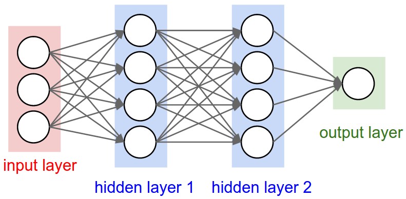
The image was taken from Andrej Karpathy’s fantastic CS 231 course. We can keep adding hidden layers to make the model as deep as needed. Note that not much changes when we make the model more complex. We can even bolt additional inputs, outputs, or whatever else we’d like and the training procedure will remain the same. That’s a pretty remarkable!

In grad school, I learned about something called “The Law of the unconscious statistician”, which is a playful way of saying all a statistician does is compute expectations by integration. There is probably a corresponding “Law of the Unconscious Machine Learner”, which states that all a machine learner does is take the derivative of the loss function and minimize. In equation form, it would probably be:

$$argmin_w \mathcal{L}(w;x,y)$$

To recap: MLPs are just logistic regression where a set of nonlinear features are automatically learned from data. You have to choose several parameters when constructing an MLP:

• Number of hidden units in each layer
• Number of hidden layers in the network
• The nonlinear activation function
• Learning rate for to use in SGD

Linear Algebra, Graphs, and Automatic Differentiation

When we derived logistic regression and MLPs, we talked things in terms of individual sums and hidden units. It turns out, however, that all of those operations can be written in terms of big matrix-matrix or matrix-vector multiplications. That’s great, because people have spent a lot of time trying to make matrix multiplcations as fast as possible. Even better, there are great GPU libraries that have ported those same innovations in linear algebra and made them available on the GPU. So we can write out everything in terms of matrix operations, move our data and model to the GPU and get huge speed ups.

But wait, there’s more! Since the chain rule/backprop effectively compartmentalizes our model components, we can use things like automatic differentiation to avoid ever having to calculate a gradient again, though you should definitely still understand how it works. There are a lot of frameworks now that will give you auto diff + GPU computation out of the box, but tensorflow is probably the most popular if you go by github stars. Here is a pretty gif of tensorflow in action:

It’s hard to express what a productivity multiplier automatic differentiation is if you’ve never had to do it the hard way. AD is very much like a compiler for machine learning models. If you were a software engineer, you can imagine much less you would get done if you still had to write everything in assembly, not to mention how many more bugs would be introduced as a result. Computer science has fundamentally always been about abstractions, so it’s nice that machine learning finally has one of its own.

AD and tensor-based graph languages allow us to specify at a high-level the important structural properties of our models, without having to compute by hand all of the derivatives by hand. In grad school, I spent countless hours in front of a white board applying the chain rule to derive the gradient and then countless more hours doing numeric checks to make sure my implementation was correct.

Don’t worry, I’m not bitter.

Implementation

So how do you actually build your own MLP? There are several ways, but my suggestion is to start with keras with a tensorflow backend. Keras seems to be at the right level of abstraction, giving you enough control to experiment while giving you a decent amount syntactic sugar so that you can learn quickly. As an added bonus, many of the default parameter settings are reflective of the current state of the art, which can save you time and agony from having to set these yourself.

The best way to learn is to try and build a model and see what breaks. Unfortunately, this means you’ll probably need access to GPU infrastructure, which can be expensive. There are some relatively cheap could options, like Amazon AWS and Google Cloud, or you could shell out a couple hundred box for a modest desktop card. As you’re getting started, a smaller card will be fine as it’s unlikely you’ll be building big, industrial grade models.

Summary of Key Terminology

That’s it for this post. Here is a handy glossary to help you keep everything straight:

• Hidden Unit - A function that takes an input (e.g. variables from data or the output of a previous layer) and performs a weighted sum followed by an application of the activation function.
• Activation Function - Transformation of a hidden unit’s output, most often nonlinear. Modern activation functions usually are a member of the “LU” family and include Rectified Linear Units (ReLU), Parametric Rectified Linear Unit (PReLU), and Exponential Linear Units (ELU). For what it’s worth, I almost always stick with the standard ReLU, as I haven’t had much success with its more esoteric cousins.
• Layer - A collection of hidden units at the same level in the graph. Takes a vector of inputs and produces a vector of outputs, where the size of the output is equal to the number of hidden units in the layer.
• Regularizaton - Methods to combat overfitting, including dropout and penalties on the $l1$ and $l2$ norms of the weights.
• Loss Function - The function to be minimized and the starting point for the backprop algorithm, usually determined by the specifics of the problem. Popular choices are binary cross entropy for 2 class classification, categorical cross entropy for multiclass classification, and mean-squared error for regression.
• Batch size - Size of each mini-batch used in computing gradients for SGD.
• Optimizer - Variant of SGD to use.
• Learning Rate - Step size to be used in SGD.

Sensible Defaults for Network Parameters

Note these are not hard and fast rules and may be wildly inappropriate for your problem. These are ballparks figures for where I usually start when working on a new problem.

• Number of hidden units - 128 - 256 to start until I get a sense of how complex the input-output relationship is, but can often go way higher to 1024 - 4096. If the network is overfitting badly on held out data, I will decrease and if it is under-fitting on the training data I will increase. I usually end up sticking with a single number that appears to be big enough and modulating the complexity of the network by adding or removing layers.
• Activation Function - ReLU. This one’s pretty easy, I always go with ReLU first and usually end up sticking with it.
• Number of layers - I usually start with 1 - 2 hidden layers and add and remove as I continue to explore. If it looks like adding more layers hurts performance on the training data, I will often see if adding residual connections between layers helps.
• Regularization - A dropout rate of 0.5 between decently big layers (~ 1024 units) and a lower rate around ~0.2 if the layers are smaller. I don’t usually use $l1$ or $l2$ penalties, but if I do it’s something small like 1e-4. Typcially do not use batch normalization either, I haven’t found it to be useful and can make training weird if you use it in the wrong place.
• Optimizer - Usually start with ADAM because it seems to work decently well off the shelf for a lot of problems. Once I hone in on a useful set of network parameters and architecture, I will experiment to see if SGD + nestrov momentum or RMSProp work better.
• Learning Rate - 1e-3 to 1e-5 seems to be a good place to start. I usually start on the high-end and if the network has trouble learning (e.g. training loss doesn’t go down or bounces wildly), I’ll turn down the learning rate and try again.
• Batch size - Depends on problem size and GPU memory, but I typically start with 64-128
• Data Scaling - Center and scale each column. Neural nets like data be be near 0 and not have many large values.

Additional Resources

• Tensorflow playground - An amazing interactive tool that visualizations various aspects of training MLPs. Take note of how much easier it is to train a ReLU network than Tanh or sigmoid ones.
• Alex Wiltschko’s great talk (and slides) on how automatic differentiation is the machine learning abstraction we have all been searching for.
• This awesome, online, and interactive online book from Michael Nielson has a ton of great reference material. Lots of great interactive demos that help illustrate concepts. Convince yourself that neural nets are universal approximators with this great visualization
• Nando de Freitas’s lecture on logistic regression as a simplified neural network. Other lectures in Nando’s machine learning course are likewise terrific.
• CS231n at Stanford - One of the best conceptual introductions to neural nets available anywhere on the internet. The entire first module covers MLPs.