June 04, 2017 / by / In deeplearning

You can probably use deep learning even if your data isn't that big

tl;dr: A hot take on a recent ‘simply stats’ post. You can still use deep learning in (some) small data settings, if you train your model carefully.

Over at Simply Stats Jeff Leek posted an article entitled “Don’t use deep learning your data isn’t that big” that I’ll admit, rustled my jimmies a little bit. To be clear, I don’t think deep learning is a universal panacea and I mostly agree with his central thesis (more on that later), but I think there are several things going on at once, and I’d like to explore a few of those further in this post.

Jeff takes a look at the performance of two approaches to classify handwritten 0s vs. 1s from the well known MNIST data set. He compares the performance of a 5-layer neural net with hyperbolic tangent activations to the Leekasso, which just uses the 10 pixels with the smallest marginal p-values. He shows, perhaps surprisingly, that the Leekasso outperforms the neural net when you only have a dozen or so samples.

Here is the figure of merit:

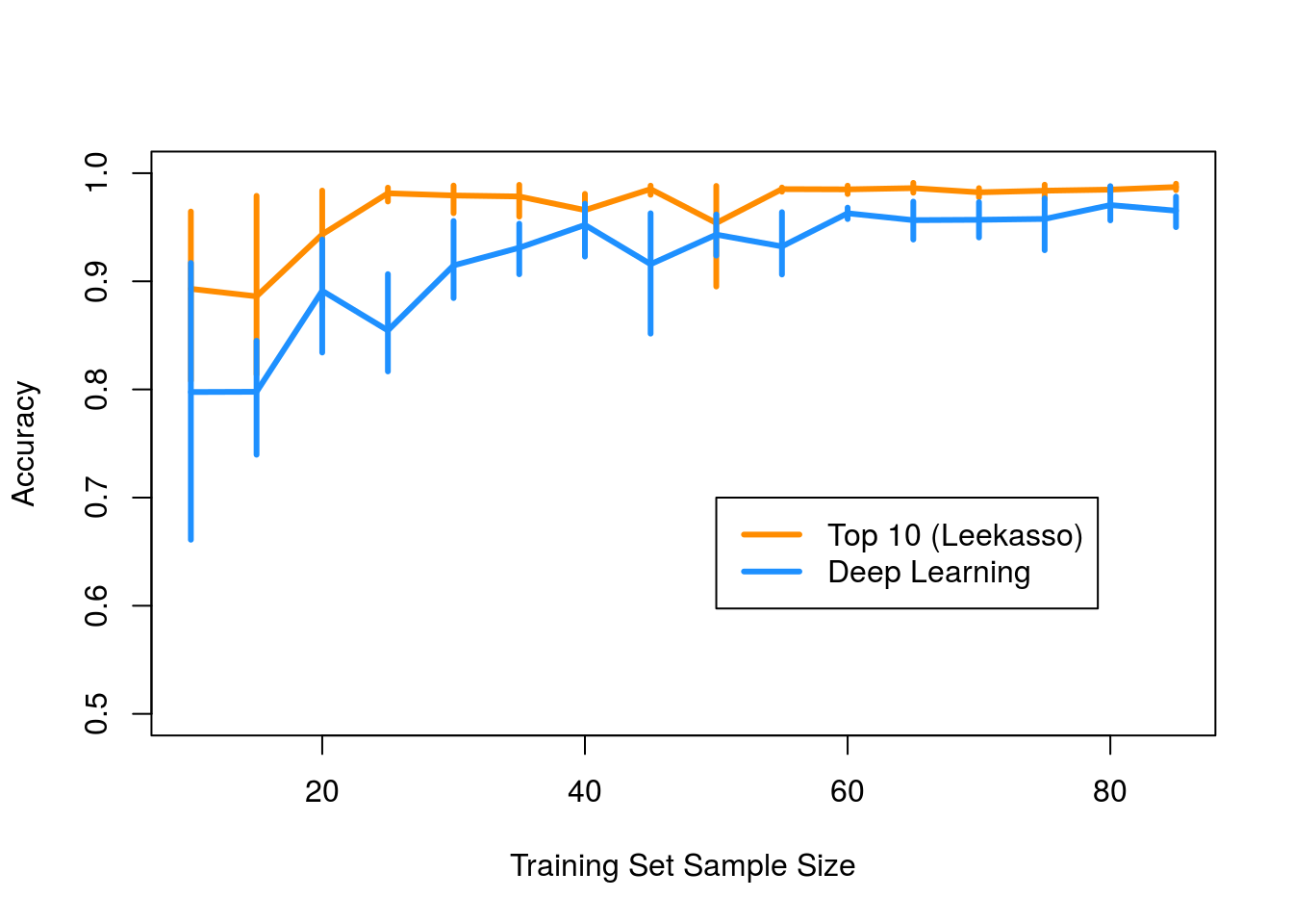
So that’s it right? Don’t use deep learning if you have < 100 samples because the model will overfit and you will get bad out of sample performance. Well, not so fast. I think there are several things going on here that are worth unpacking. Deep learning models are complex and tricky to train, and I had a hunch that lack of model convergence/difficulties training probably explained the poor performance, not overfitting.

Deep Learning vs. the Leekasso Redux

The first thing to do is to build a deep learning model someone would actually use on this data, namely modern versions of multilayer perceptrons (MLPs) and convolutional neural networks (CNNs). If the thesis of the original post is correct, these models should overfit badly when we only have a few samples.

We built a simple MLP with relu activations and a VGG-like convolutional model to see how they perform relative to the Leekasso. All of the code is available here. Big thanks to my awesome summer intern Michael Chen who did the heavy lifting and implemented most of this using python and Keras.

The MLP model is pretty standard and looks like this:

def get_mlp(n_classes):
    model = Sequential()
    model.add(Dense(128, activation='relu',input_shape=(784,)))
    model.add(Dropout(0.5))
    model.add(Dense(128, activation='relu'))
    model.add(Dropout(0.5))
    model.add(Dense(n_classes, activation='softmax'))
    model.compile(optimizer='Adam',
                  loss='categorical_crossentropy',
                  metrics=['accuracy'])
    return model

and the CNN will also look familiar to anyone who has worked with these models before:

def get_cnn(n_classes):
    model = Sequential()
    model.add(Convolution2D(32, 3, 3, activation='relu', input_shape=(28,28,1)))
    model.add(Convolution2D(32, 3, 3, activation='relu'))
    model.add(MaxPooling2D())
    model.add(Convolution2D(64, 3, 3, activation='relu'))
    model.add(Convolution2D(64, 3, 3, activation='relu'))
    model.add(MaxPooling2D())
    model.add(Flatten())
    model.add(Dense(128, activation='relu'))
    model.add(Dropout(0.5))
    model.add(Dense(n_classes, activation='softmax'))
    model.compile(optimizer='Adam',
                  loss='categorical_crossentropy',
                  metrics=['accuracy'])
    return model

For a point of reference, the MLP has about $120,000$ parameters while the CNN has nearly $200,000$! According to the hypothesis in the original post, we are going to be really screwed when we have this many parameters and only a handful of samples.

We tried to mirror the original analysis as closely as possible - we did 5-fold cross validation but used the standard MNIST test set for evaluation (about $2,000$ validation samples for 0s and 1s). We split the test set into 2 pieces. The first half was used to assess convergence of the training procedure while the second half was used to measure out of sample predictive accuracy. We didn’t really even tune these models, but just went with sensible defaults for most of the parameters.

We recreated python versions of the Leekasso and MLP used in the original post to the best of our ability, and the code is available here. Here are the out of sample accuracies for each model. The bottom plot is just a zoom-in of the best performing models to make it easier to read:

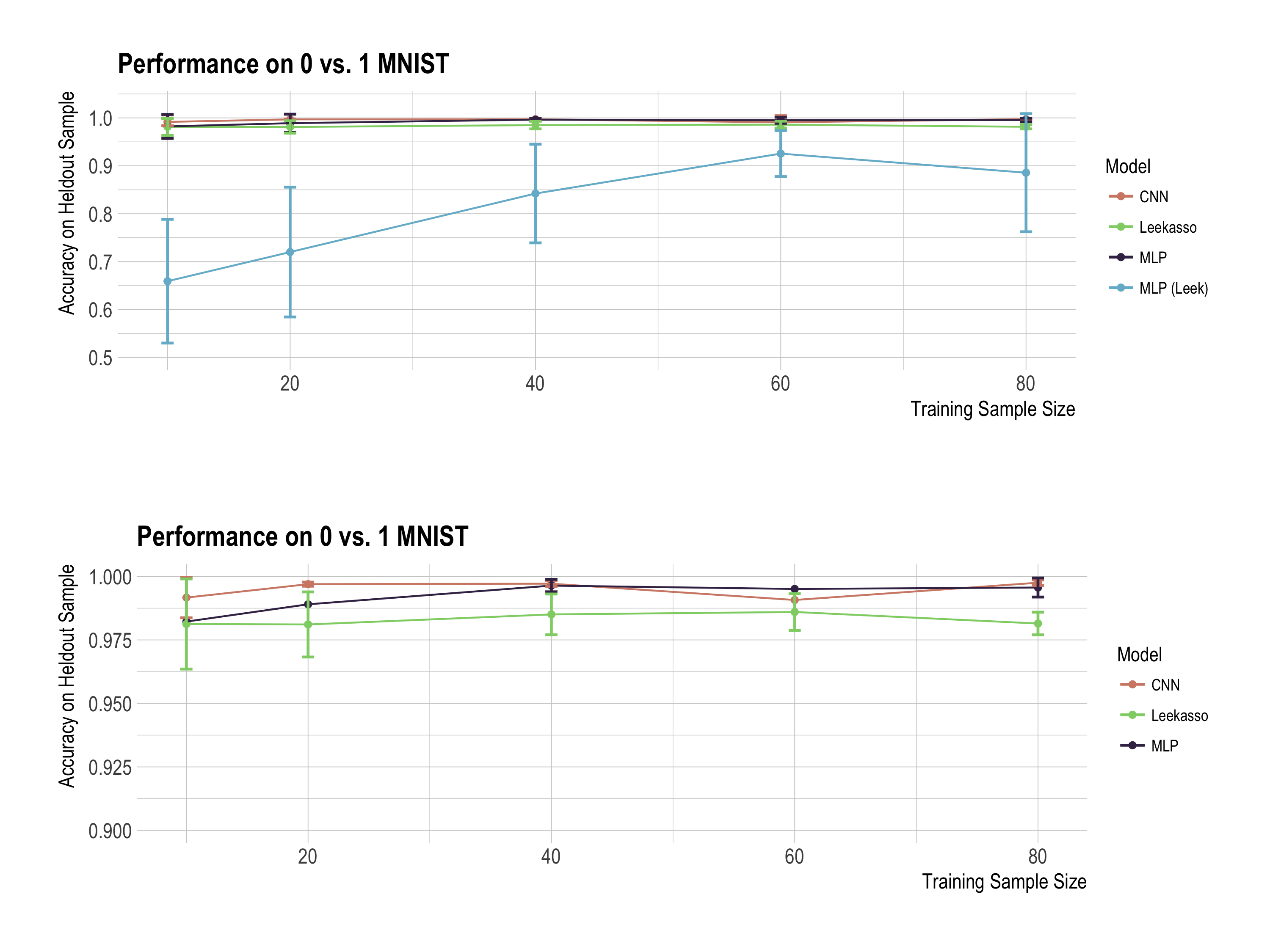
Wow, this looks pretty different than the original analysis! The MLP used in the original analysis still looks pretty bad for small sample sizes, but our neural nets get essentially perfect accuracy for all sample sizes. This all leads to the question…

What’s going on here?

Deep learning models are notoriously finicky to train, and knowing how to ‘babysit’ them is an important skill. A lot of parameters are problem specific (especially the parameters related to SGD) and poor choices will result in misleadingly bad performance. You should always keep this in mind when working on a deep learning model:

Model details are very important and you should be wary of blackbox calls to anything the looks like deeplearning()

Here are my best guesses at what is going on in the original post:

• Activation functions are very important and tanh networks are hard to train. That’s why the field has largely moved to the ‘relu’ family of functions.
• Make sure that stochastic gradient descent has converged. In the original comparison, the model was trained for only 20 epochs, which probably isn’t enough. With only $n = 10$ samples, $20$ epochs results in only $20*10 = 200$ total gradient updates. One pass over the full MNIST dataset is equivalent to $60,000$ gradient updates, and it’s common to do hundreds or thousands of passes, roughly ~ $1,000,000$ gradient updates. If you are only going to perform $200$ gradient updates, you will probably need to use a very large learning rate or your model will likely not converge. The default learning rate for h2o.deeplearning() is 0.005, which is likely way too small if you are only doing a few updates. The models we used were trained for 200 epochs and we witnessed significant fluctuation in the out of sample accuracy during the first 50 epochs. If I had to guess, I would say lack of model convergence explains most of the difference observed in the original post.
• Always check default values for parameters. Keras is nice because the default parameters are an attempt to reflect current best practices, but you still need to make sure the parameters you’ve selected are good for your problem.
• Different frameworks can give you very different results. I attempted to go back to the original R code to see if I could get the results to line up. However, I was never able to get the h2o.deeplearning() function to produce good results. If I had to guess, I would say it’s related to the optimization procedure it uses. It looks like it’s using elastic averaging SGD to push the computation onto multiple nodes to speed up training. I don’t know if this breaks down when you only have a few samples, but that would be my best guess. I don’t have a ton of experience using h2o, so maybe someone else can figure this out.

Thankfully, the good folks at RStudio just released an R interface to Keras, so I was able to recreate my python code in pure R. The MLP we used before looks like this implemented in R:

model <- keras_model_sequential()
model %>%
  layer_dense(units = 128, input_shape = c(784), activation = 'relu') %>%
  layer_dropout(0.5) %>%
  layer_dense(units = 128, activation = 'relu') %>%
  layer_dropout(0.5) %>%
  layer_dense(units = 1, activation = 'sigmoid') %>%
  compile(
    optimizer = optimizer_adam(lr=0.001),
    loss = 'binary_crossentropy',
    metrics = c('accuracy')
  )

model %>% fit(as.matrix(training0[,-1]), as.matrix(training0[,1]),
              verbose=0, epochs=200, batch_size=1)

score <- model %>% evaluate(as.matrix(testing[,-1]), as.matrix(testing[,1]),batch_size=128,verbose=0)
deep[b,i] <- score[[2]]

I dropped this into Jeff’s R code and regenerated the original plot. I changed the Leekasso a bit too. The original code used lm() (i.e. linear regression) which I found strange, so I switched it to glm() (e.g. logistic regression). The new plot is shown below:

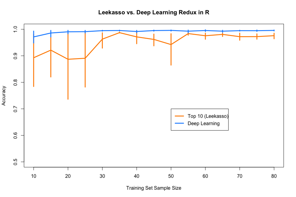
Deep learning redemption! A similar phenomenon probably explains the difference between the python and R versions of the Leekasso. The python version of logistic regression uses liblinear as its solver, which I would would guess is a little more robust than the default solvers in R. This probably matters since the variables selected by the Leekasso are highly collinear.

• This problem is too easy to say anything meaningful. I reran the Leekasso but used only the top predictor and the results are nearly identical to the full Leekasso. In fact, I’m sure I could come up with a data-free classifier that has high accuracy. Just take the center pixel and if it’s black predict $1$, else predict $0$. As David Robinson pointed out:

David also showed (in an aspirational piece of dplyr wizardry) that most pairs of numbers can be classified by a single pixel. So, it’s unlikely that this problem will give us any insight into a ‘real’ small data scenario, and conclusions should be taken with an appropriate grain of salt.

Misconceptions On Why Deep Learning Works

Finally, I wanted to revisit a point Jeff made in the original post, specifically this statement:

The issue is that only a very few places actually have the data to do deep learning […] But I’ve always thought that the major advantage of using deep learning over simpler models is that if you have a massive amount of data you can fit a massive number of parameters.

This passage, especially the last part, is not the whole story in my opinion. Many people seem to think of deep learning as a huge black box with a ton of parameters that can learn any function, provided you have enough data (where enough is some where between a million and Graham’s number of samples). It is of course true that neural networks are extremely flexible, and this flexibility is part of the reason for their success. But this can’t be the only reason they work, right?

After all, there is a 70+ year history of super flexible models in machine learning and statistics. I don’t think neural nets are a priori any more flexible than other algorithms of similar complexity.

Here’s a quick run down of some reasons why I think they’ve been successful:

• Everything is an exercise in the bias/variance tradeoff. Just to be clear, the actual argument I think Jeff is making is about model complexity and the bias/variance trade off. If you don’t have a lot of data it’s probably better to go with a simple model (high bias/low variance) than a really complex one (low bias/high variance). I think that this is objectively good advice in most cases, however…
• Neural nets have a large library of techniques to combat overfitting. Neural nets are going to have a lot of parameters, and to Jeff’s point, this will result in really high variance if we don’t have enough data to stably estimate values for those parameters. The field is very aware of this problem and has developed a lot of techniques aimed at variance reduction. Things like dropout combined with stochastic gradient descent result in a process that looks an awful lot like bagging, but over network parameters instead of input variables. Variance reduction techniques like dropout are baked into the training procedure in a manner that is difficult to replicate for other models. This let’s you train really big models (like our MLP with $120,000$ parameters) even if you don’t have a ton of data.
• Deep learning allows you to easily incorporate problem specific constraints directly into the model to reduce variance. This is the most important point I wanted to make and I think gets overlooked too often. Due to their modularity, neural nets let you incorporate really strong constraints (or priors if you prefer) that can drastically reduce the model’s variance. The best example of this is in a convolutional neural network. In a CNN, we actually encode properties about images into the model itself. For instance, when we specify a filter size of 3x3, we are directly telling the network that small clusters of locally-connected pixels will contain useful information. Additionally, we can encode things like the translation and rotation invariance of images directly into the model. All of this serves to bias the model towards properties of images to drastically reduce variance and improve predictive performance.
• You don’t need Google-scale data to use deep learning. Using all of the above means that even your average person with only a 100-1000 samples can see some benefit from deep learning. With all of these techniques you can mitigate the variance issue, while still benefitting from the flexibility. You can even build on others work through things like transfer learning.

To sum up, I think the above reasons are good explanations for why deep learning works in practice, more so than the lots of parameters and lots of data hypothesis. Finally, the point of this post wasn’t to say Jeff’s message was wrong, but to offer a different perspective on his main thesis. I hope others will find it useful.