August 20, 2016 / by / In deeplearning , convolutional neural nets , medical imaging

Segmenting the Brachial Plexus with Deep Learning

tl;dr: We competed in an image segmentation contest on Kaggle and finished 17th. Here is an overview of our approach.

Every summer our department hosts several summer interns who are considering graduate studies in biomedical informatics. This summer I had the great pleasure of supervising Ben Kompa who worked on several projects, including a Kaggle contest where we were challenged to detect and segment the brachial plexus in ultrasound images. This being a contest involving images, our approach naturally centered on the use of deep convolutional neural networks. It ended up being a close contest and we landed in the 17th spot of 923 teams and were within ~3% of the top teams. We had a lot of fun and learned a lot during the contest. Below is an overview of our experience.

Overview

The goal of the contest was to predict which pixels of an ultrasound image contain the brachial plexus. The contest is reflective of a larger trend in which AI (mostly deep learning) is starting to be used in radiology to automate some tasks. Indeed, Kaggle has had a few medical image challenges recently, so I expect this trend will continue for the foreseeable future.

For this challenge, we were given 5,635 training images (as 420x580 .tiffs) where the brachial plexus had been annotated by a person and we had to predict the pixel-by-pixel location of the brachial plexus for 5,508 testing images. In other words, this was an image segmentation challenge where the pixels in each image belonged to one of two possible classes: nerve vs. not nerve. Our task was to predict which of the possible 243,600 pixels were part of the brachial plexus for each image in the test set. Agreement between actual and predicted masks was measured using a modified form of the Dice coefficient. To be concrete, let $y_i = <y_{i1},..,y_{in}>$ be the binary vector representing the true mask for image $i$ and $\hat y_i = <\hat y_{i1},..,\hat y_{in}>$ be the binary vector representing our predictions for image $i$, where $n = 420 \times 580 = 243,600$ pixels. The Dice coefficient for $y_i,\hat y_i$ is defined as:

$$Dice(y_i,\hat y_{i}) = \frac{2*y_i \cap \hat y_i}{\left\vert{y_i}\right\vert + \left\vert{\hat y_i}\right\vert}$$

where $2*y_i \cap \hat y_i$ is the number of pixels where $y_i,\hat y_i$ are both equal to 1 and $\left\vert{y_i}\right\vert,\left\vert{\hat y_i}\right\vert$ is the total number of positive pixels in each vector. Note that $Dice(y_i,\hat y_{i}) \in [0,1]$.

However, there were a lot of images (more than half) where the brachial plexus was not present at all (i.e. $y_i$ is all 0s), or was not thought to be present by the person who annotated the image (more on this later). Because of this, the contest actually used a modified version of the Dice coefficient that gave a perfect score of 1 if you predicted an empty mask and were correct. The actual score metric was thus:

$$Score(y,\hat y) = \begin{cases} 1 & \left\vert{y}\right\vert = \left\vert{\hat y}\right\vert = 0 \\ Dice(y,\hat y) & \left\vert{y}\right\vert > 0 \\ \end{cases}$$

Outside of this unique scoring metric, there were a few data quality issues that were discovered during the course of the contest. For instance, some competitors noticed that several of the training images appeared to have been mislabeled. Below is a representative example.

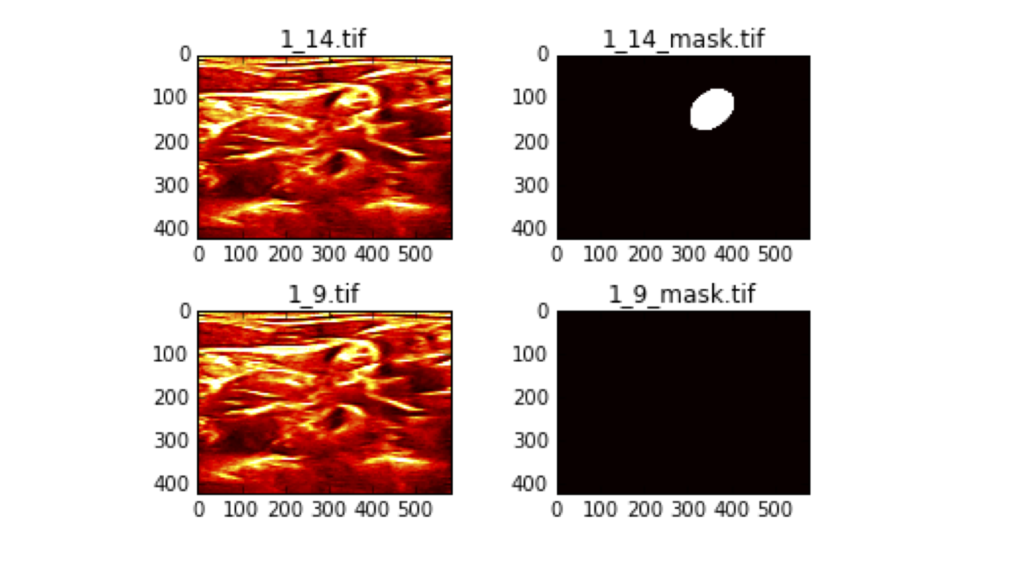
These are two images from the same patient (“1_” indicates that these are both from patient 1), that look very similar yet have completely different annotations. Annotation 1_14_mask.tif shows the brachial plexus is present in the upper right-hand corner indicated by the white circle, while 1_9_mask.tif says that it is not present at all, despite the fact that there is very little visible different between the two ultrasound images (shown on the left). This meant that the task was more like “predict what an annotator probably saw” instead of “segment the brachial plexus”.

Approach

Our final approach ended up being relatively straightforward and was designed to reduce the variance we observed in our predictions. We fit a UNET model that minimized the negative log of a smooth version of the Dice coefficient, shown below:

$$Loss(y_i,\hat p_i) = -\log \frac{2*y_i^T\hat p_i + 1}{\sum(y_i) + \sum(\hat p_i) + 1}$$

where $\hat p_i = <\hat p_{i1},..,\hat p_{in}>$ is the vector of probabilities for each pixel produced by the neural network. Note that if $\sum(y) = 0$ and $\sum(\hat p) = 0$, then the loss = 0 (i.e. the score = 1), so this gives us a nice, smooth approximation to the contest score function.

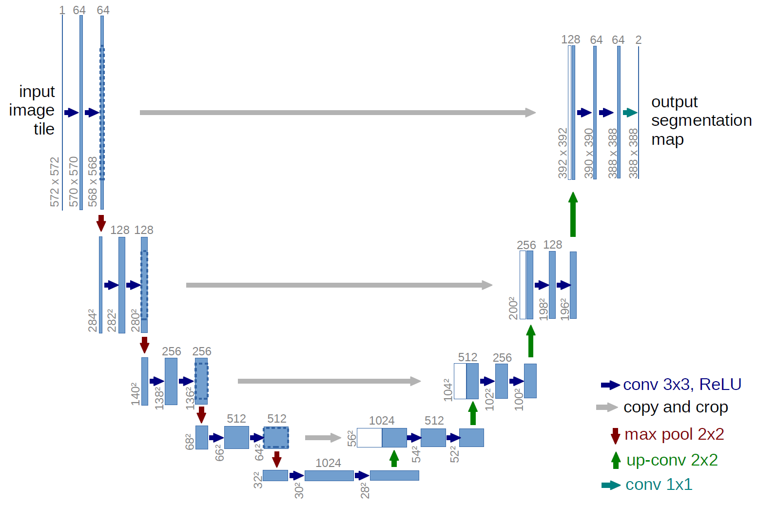
Our model was based in part on Marko Jocic’s Keras implementation. The UNET model has seen some success in image segmentation challenges (including 3rd place in the recent Data Science Bowl) and I suspect many other top teams were also using some form of the UNET. The main idea is that after each convolutional block, information travels along two pathways. One way is down a traditional down-sampling/max-pooling path that you would see in most CNNs and the other is a skip-type connection that merges with a convolutional block of the same volume, that is the result of an up-sampling path. A schematic of this from the UNET paper is shown below:

We fit models on various image sizes (64x80, 128x160, 192x240, and 256x320) and found, in general, larger images led to slightly better scores. All images were z-scored using the mean and standard deviation of the training set. We made a few important tweaks to the network such as using batch normalization on the down-sampling path and added dropout to each merge on the up-sampling path, and used the following data augmentations:

• Horizontal and vertical flips
• Horizontal and vertical shifts
• Rotations
• Shears
• Zooms

Because this was a segmentation problem (and not a classification/recognition one) the same augmentation was done to both the image and the mask during training. All models were trained using Adam with data augmentation for 100-150 epochs (the batch size ranged from 16-64 depending on the image size, due to GPU memory constraints). Most of our decisions were assessed by doing k-fold cross-validation. Importantly for this competition, the data came from individual subjects, so it was important o do subject-wise CV to get an accurate estimate of your score, as there was significant with-in subject correlation for the images. Once we had settled on a good strategy, using a single model trained on 128x160 images and setting each $\hat y_{ij} = 1$ if $\hat p_{ij} > 0.5$, we were able score 0.69 on the public leaderboard. However, we observed a lot of variance from run to run with scores ranging from 0.65 - 0.69 even with the same settings and parameters.

One of the first observations we made is that we could roughly estimate what our leaderboard score would be based on the file size of the submission. We noticed that files between 1.8MB - 2.4MB usually scored well, and anything outside this range was unlikely to receive a good score. Here’s a plot showing the relationship between file size and leaderboard score, with a smoothed estimate of the mean shown as a blue line:

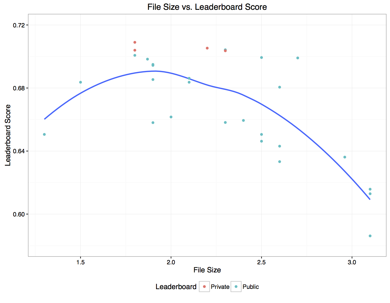
(Public scores are ones we observed during the contest and private scores are ones we measured after the contest was over.) We found we could greatly reduce this variance and improve our score by doing some simple post-processing. The smallest mask (measured by the number of active pixels) in the training set was ~2600 pixels, so it’s reasonable to assume that if the network predicts a mask with an area smaller than this value, it’s not likely that a nerve is actually present (i.e. it’s probably an empty mask). Another thing that could impact the score is the probability value that was used to set a pixel to 1, as there is no guarantee that 0.5 was optimal for this scoring metric. We did a simple cross-validation where we looked how various values for the probability cutoff and minimum mask size affected our held out validation score. This is displayed below:

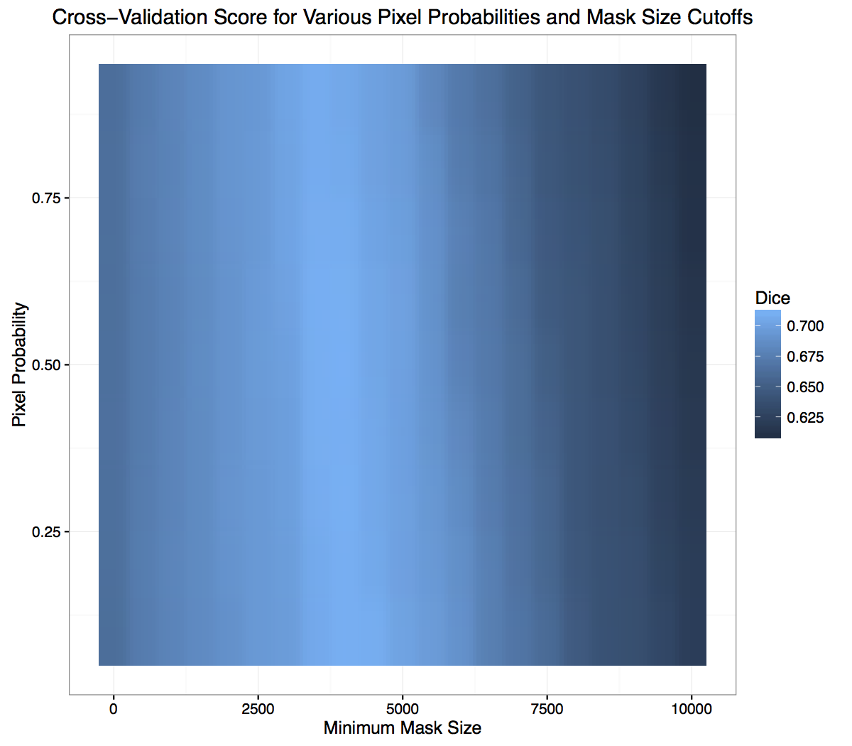
There appears to be a bright blue band (score of 0.7+) on the x-axis somewhere between 2500 - 5000 pixels, but there doesn’t appear to be a horizontal band that would indicate a similar sweet spot for the probability cutoff. Here’s the same data, but rearranged:

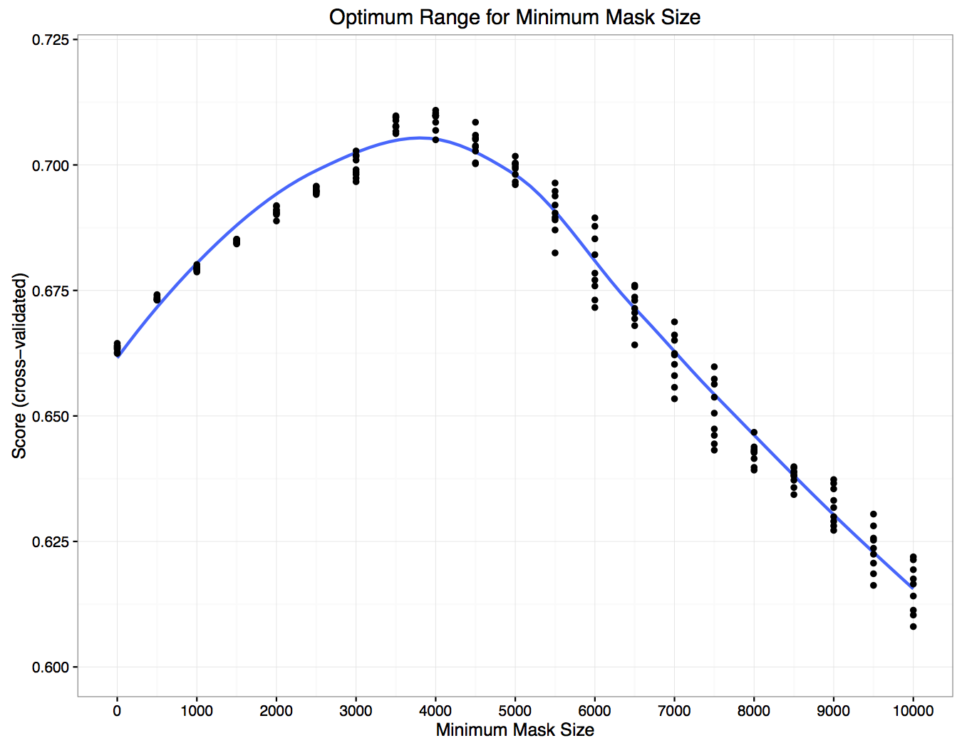
Each dot is the average held-out score for a given probability cutoff across all the folds. From this plot the minimum mask size appears to be a much more important determinant of the score than the probability cutoff, with an optimum value of ~4,000. Also, from this plot we can see that it is possible to take a raw submission (minimum mask size = 0) that would have scored 0.66 and boost it up to 0.7 by removing all masks that are smaller than ~4,000 pixels. This result was mirrored in our leaderboard submissions, and for our final submissions we used a minimum mask size of 3,500 - 4,000 and a probability cutoff of 0.8.

Summary

We were allowed to select two submissions that would determine our standing on the final leaderboard. They were:

• Single UNET model, data augmentation, 150 epochs, minimum mask size = 3500, probability cutoff = 0.8: Public score: 0.71355, Private score: 0.703
• Ensemble of two independent UNET models averaged probabilities. Image sizes of 128x160 and 192x240, data augmentation, 100 epochs, minimum mask size = 4000, probability cutoff = 0.8: Public score: 0.70074, Private score: 0.709

The ensemble model ended up being our best as judged by the final standings and landed us in 17th place. All in all, we had a lot of fun competing in this contest. It was great working with Ben who was a world-class intern and I know has a bright future ahead of him.

Things that didn’t make the final cut

As is always the case with a Kaggle contest, there was not enough time to try and implement all of our ideas. Here is an incomplete list of things we tried or wanted to try but didn’t have enough time to do:

• Classifier-coupled strategy: This was one of the more surprising parts of this contest. Early on, we trained various architectures including VGG-16 and Resnet50 to detect the presence or absence of the brachial plexus, since the scoring metric hugely rewarded you if you predicted an empty mask and were correct. We even had some fancy analysis that would take the output of both the classifier and the UNET and decide what to do based on which outcome had the higher expected value. Unfortunately, the classifier topped out at around 80% accuracy, which limited its utility. Once we started training the UNET on bigger images, the classifier was outperformed by the UNET + mask size heuristic, so we abandoned it and focused solely on improving the UNET.
• Elastic augmentation: This was also a surprising result. In the original UNET paper, the authors noted that elastic augmentation was crucial to their success, but we were unable to get any improvement from it. Since it wasn’t helping and made our training times longer, we dropped it.
• Weighted cross-entropy: Another insight claimed by the UNET paper was that using weighted pixel-wise cross-entropy as your loss function could improve things, by up-weighting the difficult pixels on the boundaries. Sadly, we never got around to seeing if it was true in this instance.
• Averaging over image augmentations: This somewhat broke my Kaggle intuitions about how it’s usually better to average over anything you can. We tried averaging over image augmentations to decrease our prediction’s variance, but this did not seem to help the final score at all.
• Training on full-sized images or full-sized crops: Because we were training on smaller 128x160 or 192x240 images, but had to make predictions for full-sized 420x580 images, we relied on cv2 in python to resize our predictions which probably isn’t optimal. We actually had room on our Titan X to train on the full-sized images, but it took a really long time and didn’t allow us to iterate quickly enough. We wanted to move towards doing random crops of the full-sized image, but never got around to it.